Computing the tangent point on the Efficient Frontier

Posted by Elliot Noma on June 16, 2017 · 1 Comment 

As noted in a previous blog post, an investor’s preferred portfolio  on the efficient frontier is determined by the point where the investor’s constant absolve risk aversion (CARA) utility function is tangent to the efficient frontier. The indifference contours of the utility function for any individual are defined by a parameter, A, which maps any investment with an uncertain return (represented by the volatility, σ and the expected return of μ) to a zero-volatility investment returning

μ– ½ * A σ²

Every point on the efficient frontier could be the preferred investment for some investor with that set of investors defined by a range of A values. When the efficient frontier is computed as a discrete set of points on the frontier, each point on the efficient frontier has an upper and lower bounds on the set of A values: the slope between the point on the efficient frontier tier an the points adjacent to it on the frontier.For instance, the following figure shows the positioning of three points on the efficient frontier where the veritical axis is the investment return and the horizontal axis is the 1/2 the variance. Given these three discrete points in the risk-return space, the middle point, M, would be the preferred investment provided A was greater than the slope of the line connecting M and U, the upper point, and less than the slope of the line connecting M and L, the lower point.

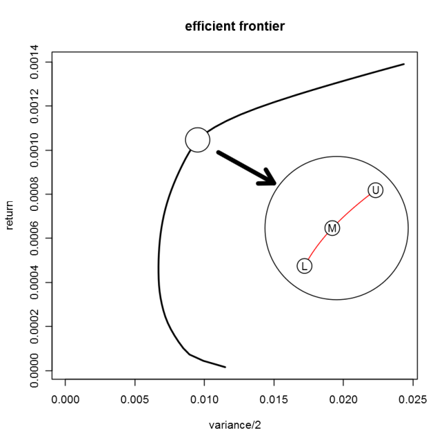
By decreasing the spacing between points on the efficient frontier, one can determine a value of A that would be associated with point M. A more practical way would be to fit a smooth curve around point M and use the first derivative of the curve at M to approximate the slope. This curve should be monotonically increasing and should have a monotonically decreasing slope as one moves from L to M to U.

 

A quadratic function fitting M and its two neighboring points, L and U will generally satisfy these conditions. To avoid square roots and keep the traditional notation of y as a function of x, we call the variance the y variable and the return the x variable in

Y = a * x² + b * x+ c

The following formulas fit the three points, L-M-U:

when

The first derivative at point M is

The inverse of this value is the first derivative at point M in terms of the original axes where the horizontal axis is the variance and the vertical axis is return. This value is the best estimate of the risk aversion coefficient, A, associate with this portfolio on the efficient frontier.

The end points of the efficient frontier can be assigned A values of infinity for the lowest volatility portfolio and zero for the highest returning portfolio.

Filed under Uncategorized